In the previous chapter we surveyed the field of visual programming.
In this chapter we create a simple visual language and explore some of
the problems that are encountered.
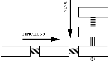
In this language every function has at most two parameters, one of which
is a function. Data flows down the vertical axis, and functions or constants
stream in from the horizontal axis.
Figure 3.1. Data andfunction concept.
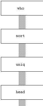
The flow of data is similar to the concepts used in the Unix operating system at the shell level, where ASCII text files can be piped into individual applications and piped out into other applications:
who | sort | uniq | head
When a command is entered at the shell level, the shell interpreter
creates pipes that handle the flow between the different programs. All
the commands may be executing at once; in effect the evaluation of the
commands is lazy.
Many of the text processing functions of an operating system fall into
the category of programs that can be written as a sequence of interconnected
commands. The shell of Unix was built to make interconnection simple. All
files were assumed to be of uniform type - newline-delimited ASCII, with
no headers.
The equivalent diagrammatic program would look like this:
Figure 3.2. Simple pipes.
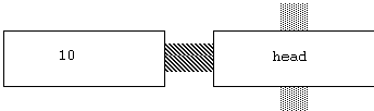
Many command functions take parameters. The function head will take a numerical argument. We consider an argument to be a constant function, and feed it in from the left side of the function box:
Figure 3.3. Arguments as constant functions.
Some aspects of the shell are quirky:
grep xyz `ls`
will yield a search of all the files in the directory for the pattern xyz.
ls | grep xyz
will search the filenames, not the contents of the files, for the pattern
xyz. In effect, the first command is applying the function grep
to all of the files. There is no clear way of indicating that a function
can be applied to a string of arguments, nor is there a clear way to use
pipes to do this.
In terms of types, we can conclude that pipes feed streams of characters,
while parameters on the command line will be interpreted as file names.
The type of an object can be interpreted by a command, which expects a
certain sort of parameter, but not by a pipe, which expects only a stream
of characters.
In trying to generate shell code from a graphic description of pipes, the problems became strongly visible. To aid both conceptualizing and coding, some form of typing system is needed.
The implied type expected by Unix text processing utilities is a sequence
of lines. Programs that work on sets of files are working on a sequence
of a sequence of lines. Lines are delimited with a line feed; files are
not delimited, but the end-of-file is detected by the operating system.
We consider here a simple type hierarchy:
| Type Name | Description | Example |
| directory | a tree containing directories as nodes and files as leaves | /usr/jeff/hyper |
| files | a sequence of files | hyper.ch1 hyper.ch2 |
| file | a sequence of lines | hyper.ch1 |
| line | a sequence of words | this is a line |
| word | a sequence of chars | this |
| char | a primitive letter | t |
In the following examples we will only use the first three types - directory,
files, file. We add the type function. We can visually show
the types of functions by keying the fill pattern of the connectors. For
example: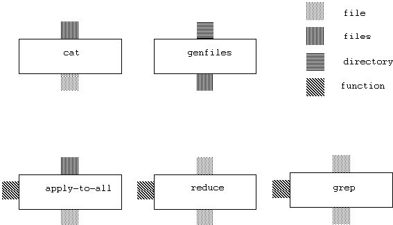 Figure 3.4. Type system.
Cat is a function that takes a stream of files and produces one
file. Genfiles traverses a directory and generates all files that
are the leaves of the tree. Apply-to-all takes files, applies a
function, and produces a single file. Reduce takes a function, applies
it to a file, and produces a file. Grep takes a file, applies a
function, and produces a file. We discuss the application of functions
next.
In a functional model, the ability to combine functions, to pass them
to other functions, is central. As an example, a sort function is
based on comparison; ideally, the comparison function should be passable
to the sort function. Likewise, the combining function apply-to-all
will take a function that operates on a type and apply it to a list of
types. Reduce will take a function and apply it to a list in such
a way as to produce a single result. In the diagram model, the functions
would be passed in from the left of the central function: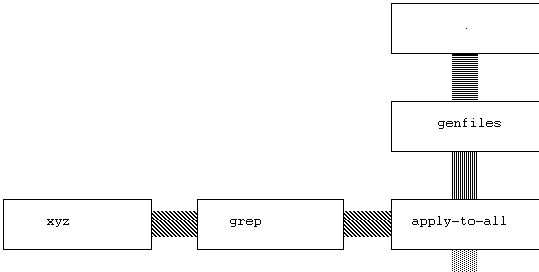 Figure 3.5. Functions as arguments to functions.
In the top box is a period; this is the Unix symbol for the current
working directory. This directory is fed into the command genfiles,
which produces a stream of files for apply-to-all. Apply-to-all
applies the command grep xyz to all of the generated files, outputting
those lines which match the pattern xyz.
It is also possible to produce mathematical output using simple functional
diagrams. The following diagram computes the factorial function by generating
a list of numbers, then reducing the list through multiplication:
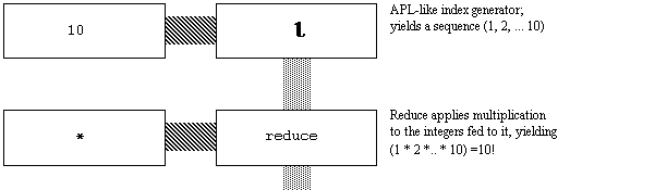 Figure
3.6. Factorial representation.
Figure
3.6. Factorial representation.
In languages such as FP, the simplicity of passing only one parameter
trades off against the clumsiness of indexing into the one parameter, which
is often a list of elements. Visual systems have this problem as well.
In the language AWK, every line is considered a set of fields. The fields can be accessed using a field number:
awk {print $1, $3}
will print the first and third fields of each line of the file that is input to it. In relational database terminology, this is a project function. Arbitrary expressions can also be created:
awk {print $1 + $3}
will print the sum of the two fields for every line in the file. This convention of using a sequence number is simple and powerful; we adopt it here as a convention. A graphic representation of an awk-like command looks like this:
Figure 3.7. Awk representation.
This means that for every line in the file, we check to see if the first
field is less than the second field. If so, we output the first field.
In database terminology, the conditional box is a select, and the
action box is a project.
A tail-recursive function on an input stream will look the same as a
conditional box. However, the semantics are different. The input stream
supplies the initial condition. The condition box supplies the test for
continuing recursion; if TRUE, then the calculation in the flow box is
done and the function is called again. For example:
Figure 3.8. Recursion.
This produces the function 2.
The single parameter is in the top box, which is combined with the initializers
in the second box. The initial value is 1, and the initial counter is set
to 0. The parameter functions as the limit on the counter. In the next
box we see the recursive computation. The initial number is multiplied
by 2, and the counter is incremented. The limit is passed through. The
counter is compared to the limit; if the counter is less, then the function
is called recursively. If the counter is equal, then the current values
are passed on to the next element in the stream, which would most likely
be a project function that would pass on the first field for additional
processing.
As the language has no variables and no loops, we use the technique
of passing counters and limits as parameters. In our recursion condition,
we check if the counter is less than the limit. If so, we recursively evaluate.
If not, the current values are the output of the function. In order to
get a single-value output, we would tie onto the end a function to project
the first field.
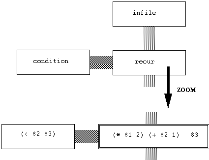
In a more complicated example (Figure 3.9), we can calculate the Fibonacci
sequence by passing the last and previous numbers in the sequence, along
with a counter and a limit. The last and previous are initialized to 1,
1, for the first two numbers in the sequence. The initial counter starts
at 2, as the next solution will be the third number in the sequence.
Note that neither this nor the previous program handle error generation
if the input is undefined, as in a negative number. They will simply produce
the initial values.
Figure 3.9. Fibonacci.
Code generation is addressed in section 3.3.2., yet it is instructive
to show here the SASL-like code generated from the above diagram:
(set datainput '((1 1 2 5)))
(set action0 (lambda (l)
  (list4 (+ (nth 1 l) (nth 2 l))
         (nth 1 l)
         (+ nth 3 l) 1)
         (nth 4 l))))
set recfunc0 (lambda (l)
  (if (< (nth 3 l) (nth 4 l))
  (recfunc0 (action0 l)) l)))

(set result (mapcar recfunc0 datainput))
(force result)
result
Note that generation of this program is relatively simple; we have a
template for a tail-recursive call, and simply fill in the condition and
the actions. As an implementation detail, we default to taking lists of
lists, so the function is invoked with a mapcar. Since evaluation
is lazy, we force it.
The interface is mouse driven, with textual and iconic menus. In many
cases the drag-and-drop convention is used - a textual object can be selected
and dragged into a function box; the object is now bound to the function.
The filenames shown are objects that can be dropped into functions, specifically
into the input box and output box functions. The bottom part of the screen
will display the output file on completion of processing.
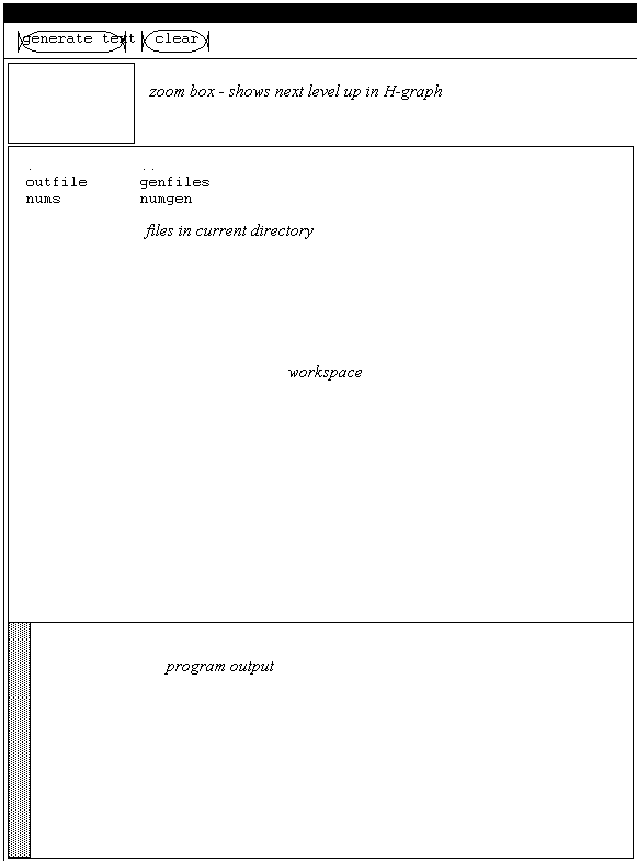 Figure
3.10. User interface layout.
Figure
3.10. User interface layout.
In order to keep every diagram simple, the concept of an H-graph is
used. Every function potentially has a graph underlying it, that can be
accessed from a zoom command. The parent of a graph can be seen through
an unzoom command. In terms of the interface, a clue as to the level in
the hierarchy is given by a miniature version of the parent graph in a
small box in the upper left.
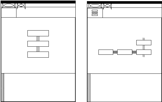
Figure 3.11. User interface zoom for H-graphs.
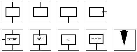
The initial graphic menu contains the boxes shown below:
Figure 3.12. Graphic menu.
On the top left is the function box; to its right are the output and
input boxes. At the far right is the parameter box. On the bottom row on
the far left is the recurrence box; when pressed it will also generate
a recursion condition box to its left. The next box is an awk box;
it will also generate a condition box. Awk is identical to recur
except that on success it does not call itself; it just passes the information
on. The box with the i in it is an index generator. To its right is the
constructor box, which will take a set of parameters and construct a list.
On the far right is the execution button.
The next figure (3.13) shows the two sets of graphic menus available.
When the mouse position is in the gray area as shown in the left screen,
outside of any function, then the menu that comes up is that show in detail
in Figure 3.12. This allows new function boxes to be added to the existing
graph. The right screen shows that when the mouse position is inside a
function box, the menu shown is one with the already defined functions
of the system. In addition, there are zoom and unzoom buttons to move to
the parent or child of the particular function the mouse is contained in.
The individual functions on the screen are shown with their text names
and types as in Figure 3.4.
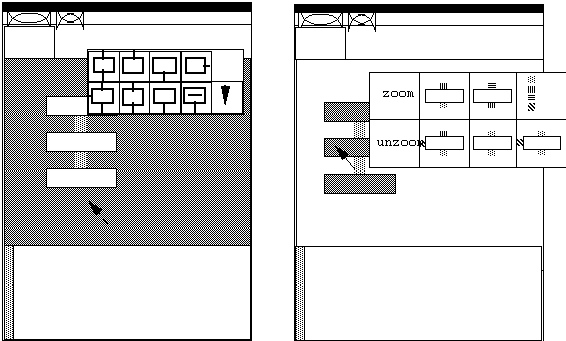
Figure 3.13. Use of menus.
A central issue in any high-level language design is what code it will generate. The visual language shown here has at different stages generated different code. The different languages generated and the problems encountered are detailed below.
The initial implementation of this system generated only shell commands,
which were then executed using the system command from within the
program. This approach has several advantages. The shell is interpreted,
so the execution of the generated program is instantaneous. Also, the features
of the shell are well suited to linking commands together. And finally,
the tools of Unix serve as a good base of functions to interconnect.
One of the problems of shell generation has already been discussed; the nonexistent typing system makes the generation of commands difficult. Also, even though there are many existing functions needed, new ones will be needed, and the shell language itself is not functional. Finally, the invocation of shell commands relinquishes monitoring or tracing control; there is no way of watching the calculations happen as there might be with a builtŁin interpreter.
In order to build more complicated filters and achieve simple database
power, awk was generated as a second stage in the code generation.
Awk provides a simple way of filtering fields, and is relatively succinct
and powerful. It is also an interpreter. However, like the shell, it has
no typing, and as it is forked off, the parent program has little tracing
or control capability.
Additionally, awk is not a functional language. It allows assignment. It also has a concept of pre and post filtering. Using the keyword BEGIN, one can specify an operation that occurs before the input is filtered, such as initializing variables. Using the keyword END, one can specify an operation that occurs after the input is filtered, such as the printing of accumulated data. Implementing these concepts are difficult in a functional framework.
The current version of the program outputs a hybrid of shell (to handle
files) and SASL (to do calculations). The version of SASL we use is not
full; it uses prefix notation, and does not allow for ZF notation.
We picked SASL for both theoretical and practical reasons. Theoretically,
it is a full functional language with lazy evaluation. Lazy evaluation
is perfect for working with streams, although we have not taken advantage
of laziness in the examples shown. Practically, source for the interpreter
is available, and simple enough to modify. As a result the execution of
a program can be traced and graphically shown, and that error conditions
can be trapped and responded to.
Sequence numbers have little mnemonic power; for example remembering
if field 3 or field 4 in a list is the cost of an item is sometimes difficult.
Relational databases handle this by binding names rather than numbers to
columns. In the case of a visual languages, the underlying tables can be
shown to prevent confusion, and the actual element of a prototype list
can be picked to make the process simpler.
In some visual languages, dataflow diagrams are used to create expressions.
This has the advantage of taking away the indirect component of field numbers
or names. However, planarity problems are often introduced. If an expression
is complicated, the result is either a tangle of lines or the creation
of some symbolic convention to overcome the planarity problem.
The program is coded in C. The SASL interpreter comes from Kamin. The
user interface is coded in Sunview.
The prototype sometimes adds a level of hierarchy that cannot be shown
in the diagrams. As an example, the recur and awk functions
are displayed initially with the words recur and awk;
when zoomed in on the actual actions and conditions can be programmed.
Figure 3.14. Hierarchy of representation.
Much of the related work was discussed in the survey of the previous
chapter. In particular, the work of Pratt (1971b) is the source of the
H-Graph convention. The streams ideas come mainly from Unix; the Kernighan
and Pike text (1984) is clearly describes Unix thinking.
For the functional interpreter, the book by Kamin(1990) was used; corresponding source was obtained off the Internet and modified for the prototype. Kamin provides a succinct summary of SASL and the reasons for creating a simple interpreter around it.